Linear Regression Maths

In this blog I will be writing about Linear Regression, that is, what is linear regression, finding best fit regression line, checking goodness of fit etc.

So without any further due lets get started.

Before we dive into Linear regression lets understand what is regression and what are its use cases.

What is Regression?

Regression is a statistical method used in finance, investing, and other disciplines that attempts to determine the strength and character of the relationship between one dependent variable (usually denoted by Y) and a series of other variables (known as independent variables).

Uses of Regression

Well there are plenty of use cases for regression but I will mention 3 major applications.

Three major uses for regression analysis are:

1.    Determining the strength of predictors

2.    Forecasting an effect

3.    Trend forecasting

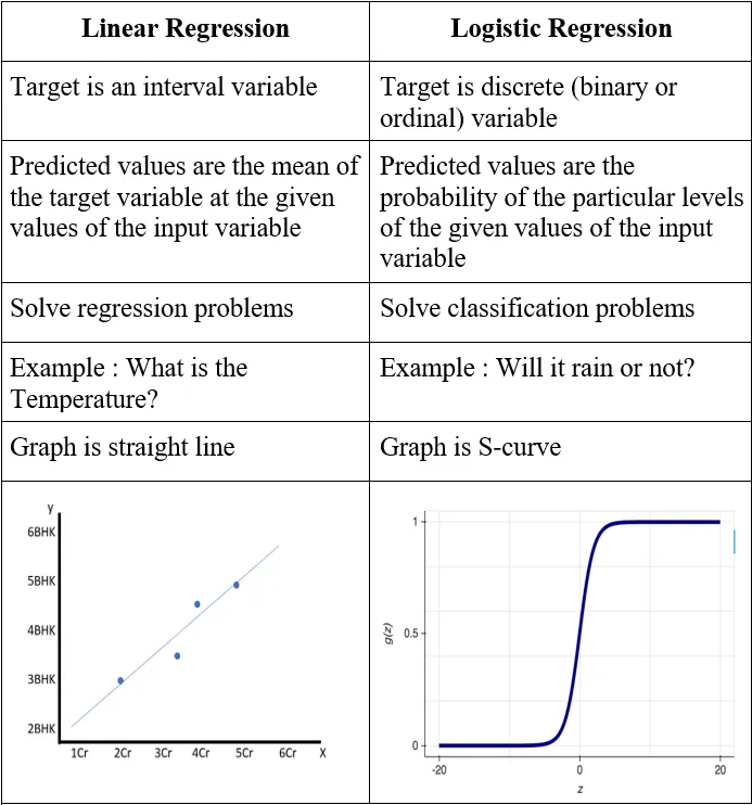
Linear vs Logistic regression

So lets get started with Linear Regression

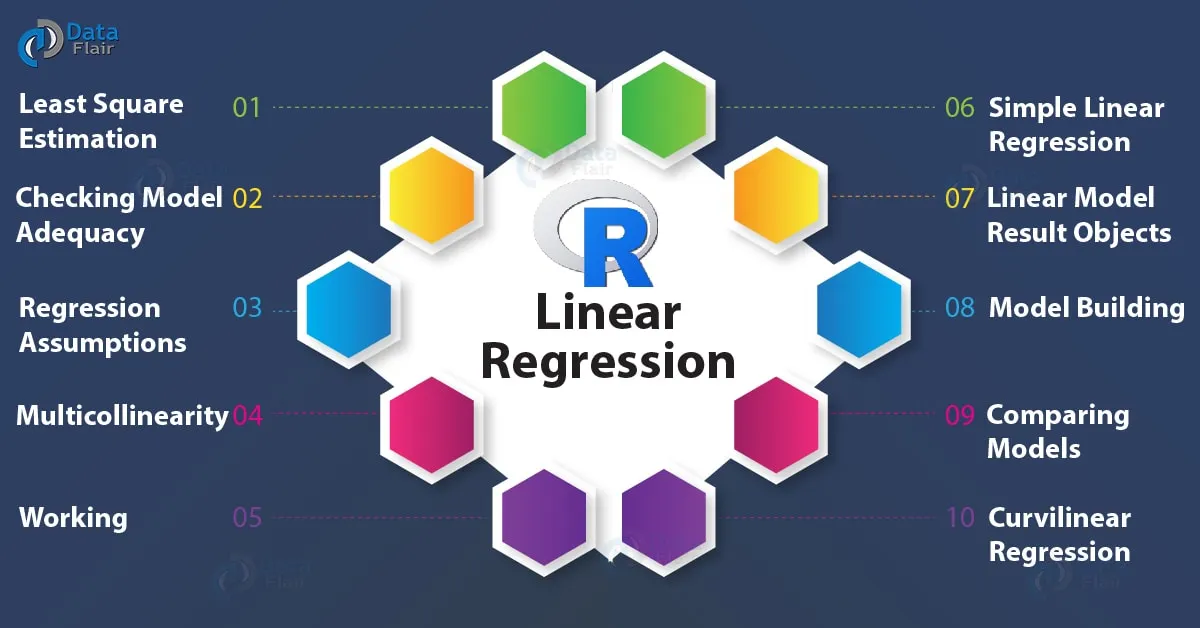
What is Linear Regression?

Linear regression analysis is the most widely used of all statistical techniques: it is the study of linear, additive relationships between variables. Let Y denote the “dependent” variable whose values you wish to predict, and let X1, …,Xk denote the “independent” variables from which you wish to predict it, with the value of variable Xi in period t (or in row t of the data set) denoted by Xit. Then the equation for computing the predicted value of Yt is:

Where Linear Regression is used?

1.    Estimating Trends and Sales Estimates

2.    Analyzing the impact of Price Changes

3.    Assessment of risk in financial services and insurance domain

Model selection for Linear Regression

In this blog I’m going to focus only on variable selection for Linear Regression, explaining three approaches which can be used:

·         Best Subset Selection

·         Forward Stepwise Selection

·         Backward Stepwise Selection

1. Best Subset Selection

This approach tries all the possible 2^p combinations of inputs with the following idea. It starts from the null model, containing only the intercept:

Then, it trains 4 models, each with only one predictor:

Finally, it picks the one with the lowest RSS or highest R² and save it.

Next, it trains other 6 models with all the possible combinations of couples of variables and then pick, again the one with lowest RSS or highest R²:

With the same fashion, for k=1,…,4, it trains each time (p k)’ (binomial coefficient) models and pick the best one (with the same criteria as before).

Then, we are left with 4 selected model with, respectively, 1, 2, 3 and 4 variables. The final step is picking the best one using metrics as Cross-Validation or adjusted error metric (adjusted R², AIC, BIC…), in order to take into consideration the bias-variance trade off.

As mentioned above, this procedure implies the estimation of 2^p different models. In our case, with only 4 variables, it boils down to the estimation of 16 models, however, with hundreds of variables it could easily get hardly feasible.

2. Forward Stepwise Selection

With forward selection, we follow a similar procedure as before, with one important difference: we keep trace of the selected model at each step and only add variables, one at the time, to that selected model, rather that estimate one new model every time.

So we start again from the null model and repeat the first step above, that is training 4 models with 1 variable each and pick the best one:

Now, instead of training 6 models, we keep the selected model and train 3 more models, looking for the one additional variable which leads to the lowest RSS or highest R².

Again, at the end of the process we will have 4 models to choose among, but the difference is that, this time, we only trained 10 models! In general, when we have p predictors, with forward selection we need to train p! models rather than 2^p.

3. Backward Stepwise Selection

The idea of this approach is similar to the Forward Selection, but in reverse order. Indeed, rather than starting from the null model, we start from the full model and remove one variable at the time, keeping trace of the previously selected model.

So, moving from the full model:

We train four different models, each obtained by removing one of the 4 predictor. Then, we select the best one with the known criteria:

From here, we train 3 models removing again one predictor at the time, but keeping fixed the model selected above:

Finally, again, we will have 4 different models to choose among. Also in this case, we need to estimate the same number of models as in Forward selection, rather than 2^p.

The main difference between Forward and Backward approach is that the former can deal with task where p>n (it simply adds a stopping rule when p=n), while the latter cannot, since the full model implies p>n.

Now to let us know about internal theory to built our Linear regression Model

Line of Best Fit

A Line of best fit is a straight line that represents the best approximation of a scatter plot of data points. It is used to study the nature of the relationship between those points.

The equation to find the best fitting line is:

Y` = bX + A

where, Y` denotes the predicted value , b denotes the slope of the line ,

X denotes the independent variable, A is the Y intercept

So, how do we find a line of best fit using regression analysis?

Usually, the apparent predicted line of best fit may not be perfectly correct, meaning it will have “prediction errors” or “residual errors”.

Prediction or Residual error is nothing but the difference between the actual value and the predicted value for any data point. In general, when we use Y` = bX +A to predict the actual response Y`, we make a prediction error (or residual error) of size:

E = Y — Y`

where, E denotes the prediction error or residual error

Y` denotes the predicted value

Y denotes the actual value

A line that fits the data “ best” will be one for which the prediction errors (one for each data point) are as small as possible.

The below diagram depicts the simple representation with all the above discussed values:

Here I will use R-Square method to calculate the closeness of the data from Best Fit Line.

What is R-Square?

1.    R-squared value is a statistical measure of how close the data are to the fitted regression line

2.    It is also known as coefficient of determination, or the coefficient of multiple determination.

Formula

The R-squared formula is calculated by dividing the sum of the first errors by the sum of the second errors and subtracting the derivation from 1. Here’s what the r-squared equation looks like.

R-squared = 1 — (First Sum of Errors / Second Sum of Errors)

First, you use the line of best fit equation to predict y values on the chart based on the corresponding x values. Once the line of best fit is in place, analysts can create an error squared equation to keep the errors within a relevant range. Once you have a list of errors, you can add them up and run them through the R-squared formula.

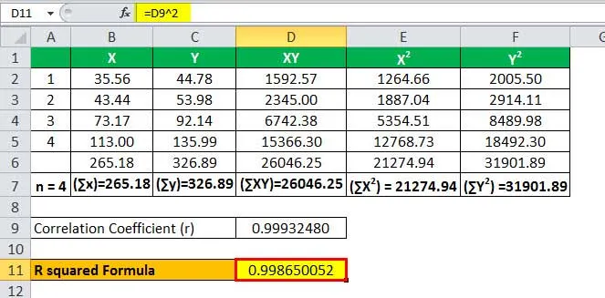
Example

Consider the following two variables x and y, you are required to calculate the R Squared in Regression.

Solution:

Using the above-mentioned formula, we need to first calculate the correlation coefficient.

We have all the values in the above table with n = 4.

Let’s now input the values in the formula to arrive at the figure.

r = ( 4 * 26,046.25 ) — ( 265.18 * 326.89 )/ √ [(4 * 21,274.94) — (326.89)2] * [(4 * 31,901.89) — (326.89)2]

r = 17,501.06 / 17,512.88

The Correlation Coefficient will be-

r = 0.99932480

So, the calculation will be as follows,

r² = (0.99932480)²

R Squared Formula in Regression

r² = 0.998650052

I tried to provide all the important information on getting started with Linear Regression and its implementation. I hope you will find something useful here. Thank you for reading till the end.