Logistic Regression (Mathematics and Intuition behind Logistic Regression)

 Data is key for making important business decisions. Depending upon the domain and complexity of the business, there can be many different purposes that a regression model can solve. It could be to optimize a business goal or find patterns that cannot be observed easily in raw data.

Even if you have a fair understanding of maths and statistics, using simple analytics tools you can only make intuitive observations. When more data is involved, it becomes difficult to visualize a correlation between multiple variables. You have to then rely on regression models to find patterns, which you can’t find manually, in the data.

In this article, we will explore different components of a data model and learn how to design a logistic regression model.

Logistic Regression

• Logistic Regression uses the sigmoid function, and this function creates a best-fitted line like an S shape.

figure 2.1 sigmoid function

• Now the question that comes into mind is that from where this function came from. so let's understand that first…
  we know the function for linear regression y=mx+c. we will just convert this function into the hypothesis form.

figure 2.2 linear equation

• but as we saw when we use linear regression to solve the binary classification problem some predicted values are greater than 1 and less than 0.but we need output values in the range between 0 and 1. how do we do this??
• we need to modify the above equation as below...

figure 2.3 sigmoid function

• The above function is our final Sigmod Function.

Let’s see how we can predict values using this sigmoid function…

We will predict X values using our sigmoid function when θ =1.

def sigmoid(x, theta=1):
    # Activation function used to map any real value between 0 and 1
    return 1 / (1 + np.exp(-np.dot(x, theta)))y_pred = sigmoid(x, 1)
y_predoutput:array([4.53978687e-05, 4.18766684e-04, 3.85103236e-03, 3.44451957e-02,2.47663801e-01, 7.52336199e-01, 9.65554804e-01, 9.96148968e-01,9.99581233e-01, 9.99954602e-01])

Now we will compare Actual values vs Predicted values by plotting the simple graph.

plt.figure(figsize=(7, 4), dpi=100)plt.ylabel('class (0 or 1)')plt.scatter(x, y, label="Actual")
plt.scatter(x, y_pred, label="Predicted")
plt.plot(x, y_pred, linestyle='-.')plt.legend()
plt.savefig('logistic_regression_12.jpg')
plt.show()

figure 2.4 actual vs predicted

Cost Function:

• Cost Function is used to check the error between actual and predicted values.
• but we don’t use the MSE function in logistic regression.
• In Logistic Regression the y is a nonlinear function, if we put this cost function in the MSE equation it will give a non-convex curve as shown below in figure 2.5.
• and when we try to optimize values using gradient descent it will create complications to find global minima.
• In Logistic regression, the Log Loss function is used as a cost function.

figure 2.5 non-convex curve

Let’s understand the Cost Function…

Below is a cost function for Logistic regression.

figure 2.6 cost function

Simplified Cost Function…

figure 2.7 simplified cost function

if y = 1 then:

this is the same as what we have in figure 2.6 when y=1

and if y = 0 then:

this is the same as what we have in figure 2.6 when y=0

After all, we have got following final Cost Function

figure 2.8 final cost function

below is a python code for the cost function:

def cost_function(x, y, t): # t= theta value
    m = len(x)
    total_cost = -(1 / m) * np.sum(
        y * np.log(sigmoid(x, t)) + 
        (1 - y) * np.log(1 - sigmoid(x, t)))
    return total_costcost_function(x, y, 1)output:
0.06478942360607087

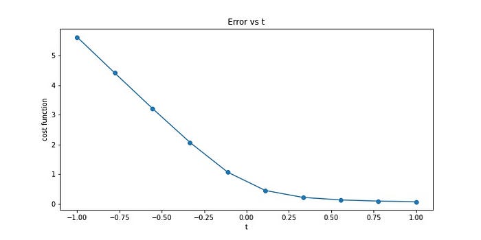
Now we will plot a graph for different values of theta

# ploting graph for diffrent values of m vs cost functionplt.figure(figsize=(10,5))T = np.linspace(-1, 1,10)
error = []
i= 0for t in T:
    
    error.append(cost_function(x,y, t)) 
    print(f'for t = {t} error is {error[i]}')
    i+=1plt.plot(T, error)plt.scatter(T, error)
plt.ylabel("cost function")
plt.xlabel("t")
plt.title("Error vs t")
plt.savefig('costfunc.jpg')
plt.show()

figure 2.9 error vs t

Gradient Descent Algorithm:

figure 3.1 gradient descent

• The Gradient Descent algorithm is the same as we saw in the Linear Regression article.
• The only difference here is the hypothesis function shown in figure 2.3
• Click here to learn about Gradient Descent.

Now it’s time for the implementation of linear regression.

Implementation:

from sklearn.linear_model import LogisticRegressionlr = LogisticRegression()
lr.fit(x.reshape(-1,1), y)
pred = lr.predict(x.reshape(-1,1))
prob = lr.predict_proba(x.reshape(-1,1))
print(y, np.round(np.array(pred), 2), sep='\n')output:
[0 0 0 0 0 1 1 1 1 1]
[0 0 0 0 0 1 1 1 1 1]

• value of theta:

lr.coef_output:
array([[0.93587902]])

• value of intercept:

lr.intercept_output:
array([-6.3343145e-17])

• final score:

lr.score(x.reshape(-1, 1), y)output:
1.0

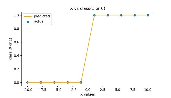
• plotting graph actual vs predicted

plt.figure(figsize=(7, 4), dpi=100)
plt.title('X vs class(1 or 0)')
plt.xlabel('X values')
plt.ylabel('class (0 or 1)')plt.scatter(x, y, label="actual")
plt.plot(x, pred, label="predicted", color='red')plt.legend(loc='upper left')
plt.savefig('logistic_regression.jpg')
plt.show()

figure 4.1

Click here for my complete Jupyter notebook on logistic regression.

Summary:

• we discuss logistic regression, cost function, and the gradient descent algorithm.
• we have understood the Intuition behind logistic regression.